How can Satellite-borne Remote Sensing Capture Crop Burning Incidents?

ISSUE BRIEF

Monitoring Crop Residue Burning Better:

Moving Beyond Fire Counts

14 October, 2025 | Clean Air

Sneha Maria Ignatious, Rishikesh P and Mohammad Rafiuddin

Suggested citation: Ignatious Sneha, Rishikesh P, Mohammad Rafiuddin. 2025. Monitoring Crop Residue Burning Better: Moving Beyond Fire Counts. New Delhi: Council on Energy, Environment and Water.

Download Study

Overview

Crop Residue Burning (CRB) is a major contributor to air pollution in the Indo-Gangetic Plain (IGP) region during winter months, particularly in October and November. Satellite-based active fire counts and burnt area are two widely used remote sensing metrics to monitor CRB. However, these methods have some limitations. Coarser spatial and temporal resolutions, as well as obstructions due to smoke and clouds, result in data loss. Moreover, these methods do not differentiate between partial burning and complete burning incidents. These limitations lead to an underestimation of CRB. An accurate estimation of CRB helps evaluate the effectiveness of its mitigation policies. Moreover, it helps in the creation of accurate emission estimates that are fed into air quality models such as Delhi’s Air Quality Early Warning System (AQEWS). Therefore, it is important to assess the effectiveness of the remote sensing methods in detecting CRB incidents and their ability to differentiate between partially and completely burnt fields.

The study analysed the effectiveness of two remote sensing-based methods - active fire counts and burnt area - in monitoring CRB. It analysed the effectiveness of satellite-borne sensors such as the VIIRS and MODIS in detecting CRB incidents. A burnt area algorithm combining two burnt area indices - Burnt Area Index for Sentinel-2 and Tasseled Cap Brightness Index (TBI) was developed to assess its ability to detect burnt fields. The study also explored the ability of this burnt area algorithm to differentiate between partially burnt and completely burnt fields.

Key Highlights

Satellite-borne sensors are unable to detect all farm fires. Our analysis of the very high-resolution satellite images shows that 169 fields were set on fire on two consecutive days over an area of 74 sq km in Sangrur in 2020. We could only find one instance where very high-resolution satellite imagery was available for two consecutive days on Google Earth. VIIRS detected only seven fires over this region, and MODIS detected none on either of the two days.
A burnt area algorithm that uses a combination of BAIS2 and TBI detected burnt pixels with 75 per cent accuracy.
Differentiating partially and completely burnt fields is challenging. The algorithm developed to separate partially and completely burnt fields could only achieve an accuracy of 60 per cent, with a high false alarm ratio of 40 per cent.
Central and state government agencies should consider using very-high-resolution satellite images to monitor CRB. However, procuring such imagery from commercial providers is expensive. Therefore, India should also move towards having its own satellites with performance comparable to that of Sentinel that complement the existing constellation. Also, air quality models should not rely only on fire count-based emission inventories, but should use burnt area-based emission inventories.

HAVE A QUERY?

Mohammad Rafiuddin

Programme Lead

mohammad.rafiuddin@ceew.in

“Crop residue burning’s impacts go beyond air quality. It impacts soil health, it releases compounds that exacerbate climate change, and the well-being of the very farmers resorting to the practice. Monitoring it is a necessity since one cannot manage what one cannot see. Given the scale of the problem, the current methods fall short, and we are left with no choice but to innovate and push the frontiers”

Executive summary

Crop residue burning (CRB) is a global concern with far-reaching environmental and public health implications. It releases greenhouse gases (GHGs), damages soil, causes air pollution, and places a significant burden on both the environment and human health (Ali et al. 2024). Despite these harmful effects, CRB remains a common method for clearing fields due to factors such as practicality, tradition, and perceptions regarding pest control. It is prevalent across countries such as Mexico, the United States, Brazil, China, and India (World Bank n.d.).

India generates around 754 million tonnes of crop residue annually, of which 228 million tonnes are surplus (MNRE n.d.). Punjab alone produces about 20 million tonnes of crop residue annually from paddy cultivation (PIB 2023b). Paddy is the leading kharif crop in Punjab, sown on around 30 lakh hectares, accounting for nearly 60 per cent of the state’s area. Farmers manage the straw generated after paddy harvest in three ways: in-situ management, ex-situ management, and burning. In-situ methods involve incorporating the straw back into the soil using machines such as the Happy Seeder and Super Seeder (Erbaugh et al. 2024). Ex-situ methods manage straw outside the fields, converting it into value-added products (ICAR 2021).

However, due to the challenges associated with these methods—such as financial constraints, limited availability of machinery, and misconceptions about the productivity impacts of residue management methods—a large share of farmers continue to practice burning. It offers the cheapest and quickest way of clearing stubble within the short window between harvest and rabi crop sowing (Erbaugh et al. 2024). This practice remains a significant contributor to air pollution in the Indo-Gangetic Plain (IGP) region, particularly during the months of October and November (Jethva et al. 2019; Lin and Begho 2022). For example, CRB contributes up to 35 per cent of PM2.5 in Delhi during the peak burning period (Govardhan et al. 2023).

Farmers burn stubble in two ways–completely or partially (Gupta 2010). In complete burning, the entire leftover straw is set on fire, whereas in partial burning, only the loose straw left after running the harvester is burnt (Kumar et al. 2015; Gupta 2010; Kemanth et al. 2024). A 2022 study found that about 58 per cent of Punjab’s farmers practised in-situ methods, but more than half of them also practised partial burning before using machines to clear their fields (Kemanth et al. 2024).

To curb CRB, the Punjab state government banned the practice in 2013 (NGT 2023). The National Green Tribunal (NGT) also prohibited it in 2015 (PIB 2019). The Union government has also introduced various schemes and issued directives to promote the use of crop residue management (CRM) machines and ex-situ management.

Crop residue burning tracking uses satellite data or on-ground observations, with satellites offering a faster and more practical option. Satellite-borne instruments such as the Visible Infrared Imaging Radiometer Suite (VIIRS) and the Moderate Resolution Imaging Spectroradiometer (MODIS) detect active fire incidents. Burnt area measurement using satellite imagery from Sentinel-2, Landsat, and other sources, or derived from MODIS and VIIRS observations, is another monitoring method. Deploying personnel on the ground and recording CRB incidents manually is labour-intensive.

Remote sensing–based methods have limitations like coarse spatial and temporal resolution, inability to see through fog, smoke, clouds, etc. Moreover, farm characteristics can change rapidly, and if the satellites pass after they change, the sensors may fail to record burning. More importantly, fire count and burnt-area methods capture the extent of CRB to a limited degree–they do not reveal whether the detected fields are burnt partially or completely.

In India, the Indian Space Research Organisation (ISRO) monitors CRB. It uses fire-count data from the VIIRS onboard the Suomi National PolarOrbiting Partnership (SUOMI NPP) and the MODIS onboard the Aqua and Terra satellites (CAQM 2021a). The National Remote Sensing Centre (NRSC) of the ISRO computes burnt area using the Mid-Infrared Burn Index (MIRBI) and publishes bulletins (NRSC-ISRO 2022). However, these burnt area data are not publicly available.

According to official fire-count data, Punjab recorded around 10,000 active fire incidents in the 2024 kharif season (CREAMS n.d.). This is the lowest since 2018, when fire counts in the state exceeded 55,000 (Kurinji and Prakash 2021). However, experts dispute these figures, arguing that farmers burn stubble after the satellite has passed overhead (NASA 2025; Misra et al. 2025). Taking cognisance of these concerns, the Supreme Court (SC) instructed the Union government and the Commission for Air Quality Management in National Capital Region and Adjoining Areas (CAQM) to obtain data from additional satellites such as the Geostationary Korea Multi-Purpose Satellite-2A (GEO-KOMPSAT-2A). Additionally, the CAQM ordered intensified patrolling during the late evening hours to monitor incidents of bypassing satellites (CAQM 2025).

This results in an inaccurate estimation of the extent of CRB. This, in turn, leads to lower emission estimates and inaccuracies in air-quality models that rely on these emission estimates for inputs. Uncertainties in both fire counts and burnt-area estimates also lead to uncertainties in understanding the effectiveness of CRB mitigation policies.

In this study, we evaluate the following questions:

To what extent do satellite-derived fire counts represent the actual extent of crop residue burning?
Can burnt area indices (indicators applied to satellite imagery to compute how much land has burned) reliably detect burnt fields, and can they differentiate between completely and partially burnt fields?

Data and methodology

We used very-high-resolution satellite imagery from the archived images available on Google Earth Pro from Maxar as the ground truth data. Of all the archived images available on Google Earth Pro between 2019 and 2025, we could only identify a region in Sangrur district, where the images were available for two consecutive days. We counted the number of fields burnt from the images and compared it with those detected by VIIRS and MODIS.

We used an algorithm that combines two indices, the Burnt Area Index for Sentinel-2 (BAIS2) and the Tasseled Cap Brightness Index (TBI), to compute burnt area from openly available Sentinel-2 imagery. We used the very-high-resolution imagery from Maxar across multiple regions in Punjab as the ground truth data to compute the accuracy of our burnt area algorithm. We propose first-of-their-kind methods to differentiate between partially and completely burnt fields. They rely on the hypotheses that either a threshold exists to differentiate between the two types of fields reliably or the number of pixels detected in a partially burnt field is lower than that in a completely burnt field.

Results

Satellite sensors are unable to fully capture the extent of fire incidents: Analysis of very high-resolution images from two consecutive days in November 2020 showed that 169 fields were either completely or partially burnt. In comparison, VIIRS detected only seven fires, and MODIS detected none, suggesting that satellite-borne sensors may not fully detect all fire events in the region. However, this is an estimate based on one instance in 2020 due to limited data availability.
Combining BAIS2 and TBI detects burnt area with 75 per cent accuracy: The study tested the effectiveness of two indices—BAIS2 (Burned Area Index for Sentinel-2), a char sensitive index which identifies burnt areas based on changes in surface reflectance, and TBI (Tasseled Cap Brightness Index), which relies on the degree of the brightness of a surface to identify burnt areas. When used together, these indices provided a more reliable classification of burnt and unburnt fields than either index alone. The combined threshold achieved a detection accuracy of 75 per cent with minimal false positives.
Differentiating between partially and completely burnt fields is more difficult than detecting burnt fields: While the algorithm designed to detect a burnt field detected burnt fields with an accuracy of 75 per cent, the proposed method, optimised for detecting only completely burnt fields, achieved only 39 per cent accuracy when applied to both types. An alternate approach—classifying fields by the number of burnt pixels—was also unsuccessful, underscoring the complexity of detecting heterogeneous burn patterns.

Limitations

While the algorithm performs well in accurately detecting burnt fields and pixels, our study has certain limitations. Missing data due to the fiveday revisit time of Sentinel-2, loss of data due to clouds and smoke, the exclusion of fields managed through in-situ methods under unburnt fields, misclassification of irrigated fields as burnt fields, and the inability to differentiate between partially and completely burnt fields, even at a very high resolution, are the limitations of this study.

Conclusion and recommendations

Our analysis of very-high-resolution satellite imagery from two consecutive days, obtained for a selected region of 74 sq km, shows that the satellite-borne fire-counting sensors detect only a portion of the fires observed in the imagery. We identified 169 burnt fields over the selected region over two days. However, the sensors could detect only seven fire incidents on these days.

Our analysis of an alternative method for monitoring CRB, including the computation of burnt area, shows that the burnt area indices BAIS2 and TBI can differentiate between burnt and unburnt fields. We observed that a combination of BAIS2 and TBI performs well with the fewest false positives. It could detect the burnt pixels with an accuracy of 75 per cent. After testing two methods to separate partially and completely burnt fields, we conclude that it is challenging to differentiate between them. Based on our learnings from the study, we recommend the following:

Central and state government agencies should use very-high-resolution satellite imagery to monitor CRB incidents, along with fire counts and burnt area. While the cost associated with satellite imagery limits extensive usage, agencies should consider using very-highresolution images from commercial satellite imagery providers, such as Maxar Technologies and Planet Labs, at least during a portion of the burning season.
The Indian Institute of Tropical Meteorology (IITM) and the India Meteorological Department (IMD) should use burnt area estimates along with fire counts to accurately estimate the emissions from CRB. Using these estimates may improve the performance of the Air Quality Early Warning System (AQEWS), which provides air quality forecasts for Delhi and other cities.
India’s future space programmes should include at least two satellites to complement the Sentinel-2 constellation. India’s own satellite constellation will enable the collection of data at a high temporal resolution, compared to the current five-day revisit time of Sentinel-2.

Introduction

Crop residue burning (CRB) is a global concern with far-reaching environmental and health impacts. It exacerbates soil erosion (Lin and Begho 2022) and reduces soil fertility by removing essential nutrients and microorganisms. It also impairs crop health (Abdurrahman et al. 2020). CRB releases harmful pollutants, such as carbon dioxide (CO2), carbon monoxide (CO), and particulate matter (PM), into the atmosphere (Pinakana et al. 2024), which impact public health adversely (TERI 2021).

Globally, farmers burn an estimated 450 million tonnes of crop residue each year (CCAC 2023). The United States ranks third in greenhouse gas (GHG) emissions from crop residues (Pinakana et al. 2024). Brazil burns about 3.2 million tonnes of rice straw annually (G. Singh et al. 2021). In Indonesia, approximately 45 million tonnes of crop residue are burnt annually (Andini et al. 2018), whereas 100 million tonnes are burnt in China (Li et al. 2022).

According to the Sardar Swaran Singh National Institute of Bio-Energy, India generates around 754 million tonnes of crop residue annually–of which 228 million tonnes is surplus (MNRE n.d.)–mainly from crops such as rice, wheat, and sugarcane. India is the second-largest riceproducing country in the world (USDA 2025), and Punjab is the fourth-largest rice-producing state in the country (UPAg, DoAFW n.d.). Farmers in Punjab predominantly follow a two-crop cycle, growing wheat during the rabi season (November–April) and paddy during the kharif season (May–October) (Kingra et al. 2017). Paddy cultivation spans approximately 31 lakh hectares (3.1 million hectares) in Punjab, yielding around 20 million tonnes of paddy straw annually (NGT 2024).

Crop residue management (CRM) methods encompass both in-situ and ex-situ approaches. In in-situ management, the stubble is incorporated back into the soil using machines such as the Super Seeder and Happy Seeder (Dhaliwal n.d.; Singh et al. 2024). In ex-situ management, the stubble gets transported off the farm and finds use in facilities such as compressed biogas (CBG) plants and thermal power plants to generate value-added products, including biogas and electricity (ICAR 2021). However, a significant proportion of farmers continue to burn straw in the field (PIB 2024). Misconceptions associated with reduced productivity from CRM machines, fears of pest attacks, the short 20–25 day window between the harvest and sowing of the rabi crop, and the higher operating costs of CRM machinery contribute to this practice (ICAR 2021; Kemanth et al. 2024). This practice of burning is a leading contributor to the increased levels of air pollution in the Indo-Gangetic Plain (IGP) region during the winter months. For instance, CRB contributes up to 30–35 per cent of Delhi’s PM2.5 during peak burning period (Govardhan et al. 2023).

To curb CRB, the central and state governments have introduced a range of schemes and measures. A brief chronology of the measures is as follows:

2013: The state government of Punjab banned CRB (NGT 2023).
2014: The Ministry of Agriculture and Family Welfare (MoAFW) launched the Sub-Mission on Agricultural Mechanization (SMAM) to extend agricultural mechanisation to small and marginal farmers and promote custom hiring centres (CHCs) (MoAFW 2018).
2015: The National Green Tribunal (NGT) also banned CRB (NGT 2023).
2018: The union government launched the Central Sector Scheme for Promotion of Agricultural Mechanization for In-Situ Management of Crop Residue. The scheme provides a 50 per cent subsidy to individual farmers and an 80 per cent subsidy to registered farmer groups, cooperative societies, and farmer producer organisations (FPOs) for the procurement of CRM machines (PIB 2021).
2018: The Ministry of Petroleum and Natural Gas (MoPNG) launched the Sustainable Alternative Towards Affordable Transportation (SATAT) scheme to encourage entrepreneurs to set up CBG plants and establish an enabling ecosystem (MoPNG n.d.).
2018: The MoPNG also launched the National Policy on Biofuels to increase the use of biofuels in the energy and transportation sectors, aiming to enable the availability of biofuels in the market to increase the blending percentage (MoPNG 2018).
2022: The Commission for Air Quality Management in National Capital Region and Adjoining Areas (CAQM) mandated all thermal power plants (TPPs) within a 300-kilometre radius of Delhi to co-fire 5–10 per cent biomass alongside coal (CAQM 2022).
2024: The MoPNG launched the Biomass Aggregation Scheme to support biomass collection for biomass-based CBG plants by providing financial assistance to CBG producers for the procurement of biomass aggregation machinery (MoPNG 2024).

Despite these efforts, Punjab recorded around 10,000 active fire incidents in 2024 (ICAR 2024). The actual number may be significantly higher, as many farmers may have started to burn stubble after the satellites pass (NASA 2025; Misra et al. 2025). Recent studies claim an increase in the adoption of in-situ machinery to manage fields, with approximately 58 per cent of farmers in Punjab adopting it in 2022. However, nearly half of them also practised partial burning before using the CRM machines (Kemanth et al. 2024). In the case of partial burning, only the loose straw left behind on the field after running the harvester is burnt; however, in the case of complete burning, all post-harvest straw is set on fire (Kumar et al. 2015; Gupta 2010; Kemanth et al. 2024).

Authorities deploy field officers and utilise two remote sensing–based metrics–active fire counts and burnt area–to monitor CRB incidents (Hindustan Times 2023). Deploying personnel on the ground and manually recording burnt fields is labour-intensive. Therefore, remote sensing methods are highly feasible. The two metrics are as follows:

Fire counts: Sensors such as the Visible Infrared Imaging Radiometer Suite (VIIRS) and the Moderate Resolution Imaging Spectroradiometer (MODIS) onboard satellites detect active fire incidents (NASA n.d.a). These sensors rely on thermal anomalies to detect fire incidents (GWIS, n.d.).
Burnt area: There are two ways of burnt area estimation. The first method utilises firecount data while the second employs burnt area indices applied to spectral measurements from satellite-borne instruments. The first method considers a fixed area surrounding the location of the detected fire as the burnt area (Ambulkar et al. 2025). The second method presupposes that the spectral signature of a field differs before and after burning. Researchers have designed various burnt area indices, such as the Tasseled Cap Brightness Index (TBI), Burnt Area Index for Sentinel-2 (BAIS2), Normalised Burn Ratio (NBR), Normalised Burn Ratio 2 (NBR2), Burn Area Index (BAI), and Mid-Infrared Burn Index (MIRBI), based on this principle (Kouadio et al. 2023).
Several researchers have attempted to compute the extent of CRB and the related challenges in India and abroad using satellite imagery, fire-count data, and ground surveys (Li et al. 2022; Mohammad et al. 2023; Singh et al. 2021; Kumar et al. 2025; Sehgal et al. 2021; Liu et al. 2019). In India, the Indian Space Research Organisation (ISRO) records and monitors fire incidents and burnt areas. It relies on VIIRS data from the Suomi National Polar-Orbiting Partnership (SUOMI NPP) satellite and MODIS data from the Aqua and Terra satellites to track active fire incidents (CAQM 2021a).
According to the burnt area estimates released by the National Remote Sensing Centre (NRSC), ISRO, Hyderabad, burnt area computation uses the burnt area index MIRBI using Sentinel-2 data (NRSC-ISRO 2022). However, Deshpande et al. (2022) have found that MIRBI’s ability to separate burnt and unburnt pixels is lower compared with that of indices such as BAIS2 and TBI. Moreover, the NRSC has not made the detailed methodology or state-level burnt area estimates publicly available.

Several uncertainties are associated with remote-sensing methods:

Coarse spatial resolution: Sensors only detect fires that are active during the satellite overpass time. The SUOMI NPP/VIIRS1 passes over the IGP region around 01:30 a.m. and 01:30 p.m. local time, while the Aqua and Terra2 satellites pass over India just after 10:30 a.m. and 01:30 p.m. (Payra et al. 2023). The revisit times of VIIRS and MODIS are 12 hours (Schroeder et al. 2014; Parkinson 2022). Satellites fail to detect fires occurring before or after the overpass times, resulting in an underestimation of fire incidents (Fusco et al. 2019). The spatial resolution of VIIRS is 375 m and that of MODIS is 1 km (NASA Earthdata 2024). Therefore, fires over areas smaller than 375 m or 1,000 m may fail to get detected by these instruments. For instance, the average size of farmland in Punjab is 4 hectares (40,000 sq m), which is smaller than the 375 m x 375 m resolution offered by VIIRS (Kurinji and Prakash 2021). In addition, small, localised fires may not result in strong enough thermal anomalies for the instruments to capture them (Jaffe et al. 2020; Zhang et al. 2021; Chen et al. 2022). Additionally, partial burning lasts only a few hours, making it difficult for satellites to detect (Kemanth et al. 2024). Studies have attempted to complement satellite data with household surveys and crop statistics to reduce uncertainties; however, this remains a significant challenge in satellite-based monitoring of CRB (Liu et al. 2020).
Coarse temporal resolution: Sentinel-2 multispectral instruments offer a spatial resolution of 10–60 m but have a revisit time of five days (ESA n.d.). Harmonised Landsat and Sentinel-2 (HLS) images are available with a temporal resolution of 2–3 days, while the spatial resolution is 30 m (NASA n.d.).
Obstructions: Clouds, smoke, and smog obscure active fire and burnt area detection using remote-sensing methods (Copernicus n.d.; Luft et al. 2022).
Surface reflectance variability: The spectral characteristics of burnt fields can vary with time (Singh et al. 2021), and longer satellite revisit times pose a challenge, as the burnt area indices may fail to detect such farms due to a change in characteristics.
Incomplete information: Both the fire count and burnt area methods cannot differentiate between partially burnt fields and completely burnt fields. Moreover, no study has attempted to distinguish between partially and completely burnt fields yet. A clear distinction between partially burnt fields and completely burnt fields is crucial for accurately estimating emissions and assessing the extent of CRM adoption.

These limitations result in an underestimation or overestimation of CRB. This, in turn, has significant consequences:

Underestimation of emissions from CRB: Emission inventories (EIs)–such as the Fire INventory (FINN) from the National Centre for Atmospheric Research (NCAR)–rely on fire counts to estimate CRB emissions (Wiedinmyer et al. 2023). Chemical transport models (CTMs), widely used to model air pollution, use these EIs as inputs to account for such emissions. For instance, India’s CTM-based Air Quality Early Warning System (AQEWS) incorporates the FINN EI to account for CRB emissions (Govardhan et al. 2024). Uncertainties also arise from differences in fuel-loading ratios and emission factors across global EIs (Hua et al. 2024). The CAQM implements the Graded Response Action Plan (GRAP) in Delhi based on AQEWS forecasts (PIB 2023a). Reliable and accurate EIs are therefore essential for accurate forecasting.
Difficulty in assessing the impact of mitigation policies: Both the union and state governments allocate significant financial resources to the policies aimed at curbing CRB. For instance, the union government spent approximately INR 3,600 crore under the Central Sector Scheme for Promotion of Agricultural Mechanization for In-Situ Management of Crop Residue between 2018 and 2024 (PIB 2025). Government sources use fire-count data to measure the success of such schemes. However, a change in fire counts should not be the sole metric to gauge the effectiveness of these policies. The Supreme Court recently noted the CAQM’s observation that farmers were bypassing satellite monitoring and that the burnt area was increasing over the years, despite a decrease in fire counts. Following this, it directed the CAQM to submit fire-count data from geostationary satellites such as the Geostationary Korea Multi-Purpose Satellite-2A (GEO-KOMPSAT-2A), not just from polarorbiting satellites (SCO 2024). Moreover, the CAQM also directed enforcement agencies to increase patrolling during the evening hours to monitor such bypassing incidents (CAQM 2025). News reports also suggest that some farmers have shifted to partial burning, resulting in a reduction in emissions from CRB (Newslaundry 2022). However, there are no scientific studies quantifying these changes.

The CAQM monitors CRB incidents using a protocol developed by ISRO (CAQM 2021b). However, as discussed earlier, farmers may have started to burn after satellite overpasses to avoid detection. Therefore, it is crucial to understand the extent to which satellite-borne sensors detect active fires and whether burnt area can complement or substitute for fire counts in monitoring CRB. It is also equally important to determine whether burnt area–based methods can capture partially burnt fields and differentiate them from completely burnt fields.

Through this study, we aim to:

Assess the extent to which the fire count–based methods capture actual burning.
Develop a methodology to compute burnt area.
Test whether burnt area methods can differentiate partially burnt fields from completely burnt fields.

Our analysis focuses on Punjab during the post-kharif harvest period, when farmers typically burn paddy residue.

Data and methodology

We used openly available VIIRS data and very-high-resolution satellite imagery to assess the extent to which CRB incidents get captured by satellite-borne sensors. Alongside, we also used Sentinel-2 multispectral imagery to develop an algorithm based on spectral indices to estimate the burnt area.

Data

We obtained fire-count data from the VIIRS instrument onboard the SUOMI NPP satellite and the MODIS instrument onboard the Aqua and Terra satellites. To identify burnt and unburnt fields for training and validating the algorithm, we relied on openly available very-high-resolution archived imagery from Maxar Technologies available on Google Earth Pro. We applied our algorithm to band data from the multispectral sensor onboard the Sentinel-2 satellites (NASA n.d.b).

Methodology

Assessing the ability of satellite-borne sensors to capture crop residue burning incidents

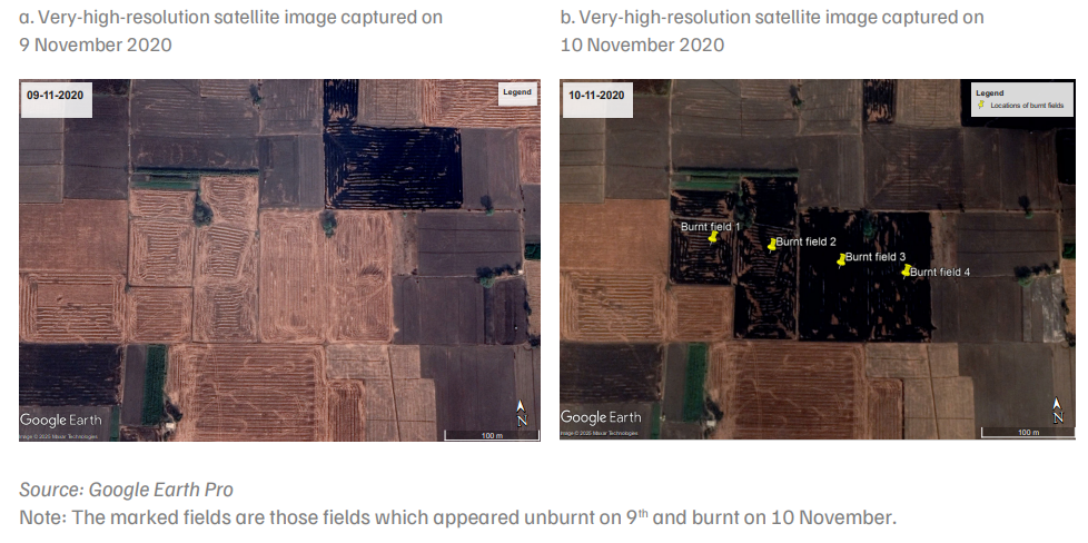
We identified a region of approximately 74 sq km in Sangrur where Google Earth Pro images were available for two consecutive days–9 and 10 November 2020. Images from the two successive days helped us identify the fields that were initially unburnt but were burnt on either of the two days. If a field that appeared unburnt appears black on the second day’s image, it implies that the field was set on fire during the interval between the image acquisition times. Among archived images available on Google Earth Pro between 2019 and 2025, we could only identify this region in Sangrur with such consecutive-day coverage.

We then visually identified the fields that were unburnt on the first day and burnt on the second day. We considered a field burnt if it appeared black or grey in the image on the second day but not on the first. An unburnt field appears golden-yellow or green in the images. Figure 1 illustrates fields from both dates over a subset of the study region, along with the fields we identify as burnt. We also obtained the locations and fire counts detected by the VIIRS instrument (at all confidence levels) over the selected region. The MODIS instruments did not capture any active fire incidents over this region on these two days. We then compared the number and locations of burnt fields identified through imagery with the active fires detected by VIIRS.

Figure 1. Very-high-resolution satellite imagery obtained for two consecutive days help identify fields burnt on each day

Assessing the performance of the burnt area indices in detecting burnt and unburnt pixels

Algorithm

Our algorithm involved applying burnt area indices to Sentinel-2 imagery to distinguish between burnt and unburnt fields. We focused on two indices–BAIS2 and TBI–and applied them to the Sentinel-2 band data to assess their ability to detect burnt fields and differentiate between completely and partially burnt fields. While BAIS2 is an ash and charcoal sensitive index which uses spectral characteristics of the red edge and short wave infrared bands of Sentinel-2, TBI is a brightness index which measures the brightness of a surface. Deshpande et al. assessed the separability index to evaluate how well different burnt area indices differentiated burnt and unburnt pixels. The study found that the separability index of BAIS2 and TBI is higher than that of indices such as MIRBI, Normalised Burn Ratio (NBR), etc (Deshpande et al 2022).

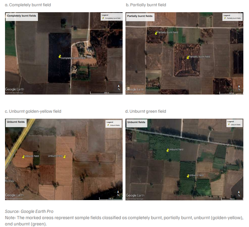
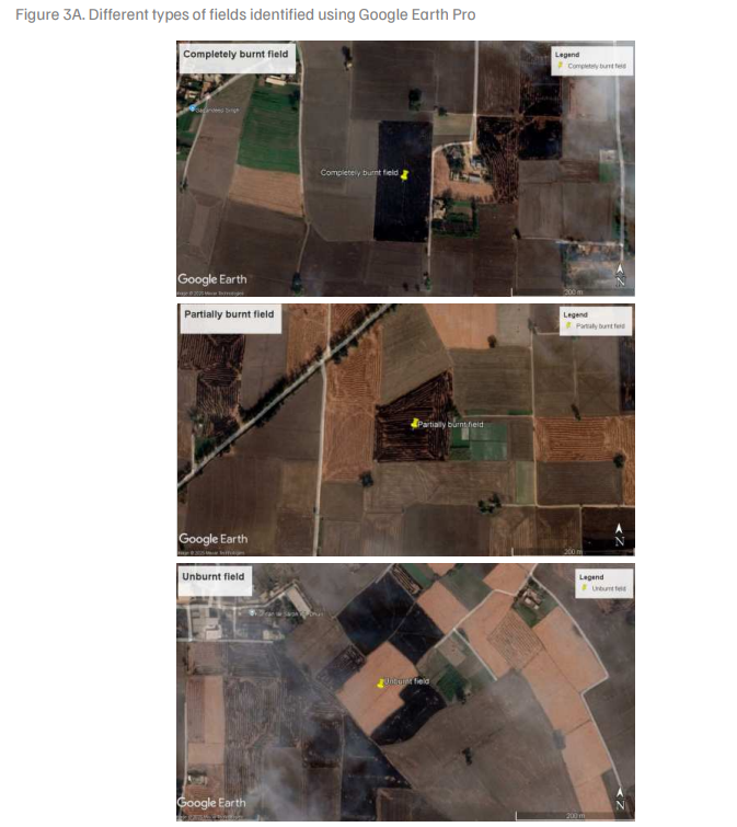
We obtained very-high-resolution satellite imagery from Google Earth Pro for dates where Sentinel-2 data are also available. We could only identify four such dates between 2019 and 2025 in Punjab during the peak burning season (between 15 October and 30 November). For the training dataset, we identified a ~220-sq km region in Sangrur where very-high-resolution imagery from Google Earth Pro and Sentinel-2 multispectral satellite imagery were available on the same date (10 November 2020). Using this imagery, we visually classified fields as partially burnt, completely burnt, and unburnt. A completely burnt field appears entirely black in the images. However, a partially burnt field appears black, interspersed with regularly spaced goldenyellow patches along its length, corresponding to the unburnt residue that is later incorporated into the soil using CRM machines. We mark two types of fields as unburnt: the ones that appear golden-yellow and those that appear green. We excluded in-situ managed fields from the unburnt category, as these were challenging to identify reliably from satellite imagery. Figure 2 illustrates the different field types.

Figure 2. In very-high-resolution satellite imagery, a completely burnt field appears entirely black, while a partially burnt field shows black areas interspersed with regularly spaced golden-yellow patches

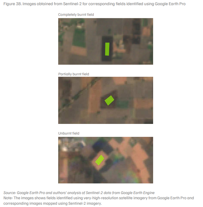
We then mapped these fields onto Sentinel-2 imagery using Google Earth Engine (GEE). We extracted the pixels from within these fields by drawing polygons within corresponding field boundaries using the Polygon drawing tool (or ‘Draw a shape’) available on GEE. We avoided the pixels along the edge of the field boundaries to prevent the inclusion of pixels from neighbouring fields. Figure 3 illustrates the sample polygons that we drew on GEE to extract the pixels. We then applied BAIS2 and TBI to the Sentinel-2 band data for these pixels. Annexure 1 explains the formula behind these indices and the spectral bands used to compute them.

Figure 3. Burnt area indices were computed from Sentinel-2 pixels for fields mapped using very-high-resolution imagery

Thereafter, we analysed the histograms of BAIS2 and TBI for pixels from unburnt, partially burnt, and completely burnt fields to identify the thresholds that could potentially separate these categories. We tested the performance of BAIS2 and TBI separately as well as together. For this, we analysed the histograms of burnt and unburnt field pixels as discussed in Deshpande et al. (2022) and set the thresholds based on percentiles. Deshpande et al. (2022) set the 5^th and 95^th percentiles of the indices as the lower and upper thresholds to avoid overlapping pixels and outliers. However, we did not cap the index values at both ends. The theoretical minimum value of TBI is zero (Annexure 1), corresponding to a perfectly black field. The BAIS2 value of burnt scar ranges between −1 and 1, and it is between 1 and 6 for active fires (Alcaras et al. 2022). Therefore, a cap on the BAIS2 values might cause the algorithm to miss fields that are actively burning. Hence, we did not cap the maximum value of BAIS2 or the minimum value of TBI.

Setting the thresholds

Our analysis of the BAIS2 and TBI values for different types of fields in the training dataset shows that both indices can potentially distinguish between unburnt and burnt fields. Figure 4 shows the histograms of BAIS2 and TBI of completely burnt, partially burnt, and unburnt pixels.

Figure 4. Tasseled Cap Brightness Index (TBI) and Burnt Area Index for Sentinel-2 (BAIS2) can potentially separate unburnt, partially burnt, and completely burnt fields

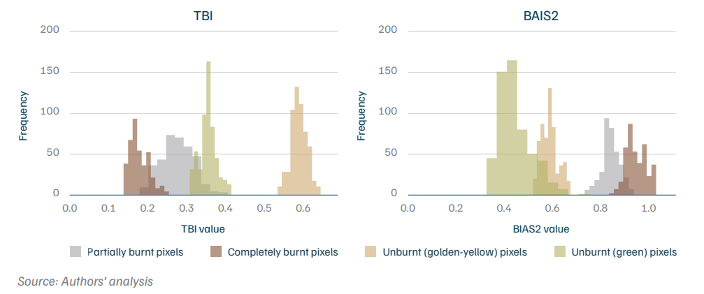
However, as Figure 4 shows, TBI values for green and burnt fields overlap, while BAIS2 values for golden-yellow and burnt fields lie close together. To test whether combining thresholds improves classification, we analysed BAIS2 and TBI jointly rather than individually. Deshpande et al. (2022) also used a combined approach, capping the values of these indices between the 5th and 95th percentiles. In our case, we selected the threshold values – T1, T2, and T3 based on the index values obtained for partially burnt fields, ensuring that our algorithm captured both partially and completely burnt fields. Table 1 lists the thresholds used.

Table 1. Thresholds tested in this study to distinguish between burnt and unburnt fields

Threshold

Description

Threshold 1 (T1)

BAIS2 >= 5th percentile value of partially burnt pixels

Threshold 2 (T2)

TBI <= 95th percentile value of partially burnt pixels

Threshold 3 (T3)

BAIS2 >= 5th percentile value of partially burnt pixels
TBI <= 95th percentile value of partially burnt pixels

From the training dataset, we identified the values of these thresholds. We have summarised the values in Table 2.

Table 2. Values of the thresholds identified from the training dataset

Threshold	Threshold value
Threshold 1 (T1)	BAIS2 >= 0.78
Threshold 2 (T2)	TBI <= 0.34
Threshold 3 (T3)	BAIS2 >= 0.78 TBI <= 0.34

Source: Authors' analysis

Validation

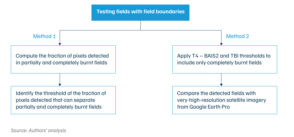
To validate the algorithm’s performance, we identified a test region in Punjab where the image dates of the very-high-resolution imagery from Google Earth Pro coincided with Sentinel-2 multispectral imagery. Suitable images were available for 29 October 2021, covering Hoshiarpur and Jalandhar. We then applied threshold T3 to 10 randomly selected villages across this region, which spans an area of approximately 28 sq km. Within these fields, we marked burnt fields and their field boundaries, extracted the pixels from within the fields, and created subsets of partially burnt, completely burnt, and unburnt fields. In total, we identified 287 burnt fields and 95 unburnt fields across the 10 villages. Of the 287 burnt fields, we could only clearly identify 72 completely burnt fields and 190 partially burnt fields.

We analysed the performance of the algorithm using two criteria:

Ability to detect burnt fields accurately: The effectiveness of our algorithm depends on how accurately it detects both partially and completely burnt fields while avoiding unburnt fields. The algorithm is said to detect a field if it detects at least one pixel within the field. This corresponds to an area of 100 sq m.
Ability to detect burnt pixels accurately: Accurate computation of burnt area requires accurate detection of all burnt pixels while minimising the detection of the unburnt ones. Using the matrix in Table 3, we computed accuracy, true positive rate (TPR), false positive rate (FPR), false negative rate (FNR), F1 score, Matthews correlation coefficient (MCC), and Cohen’s kappa (k). Table 4 presents the metrics and formulas used.

Table 3. The confusion matrix used for computing performance metrics

		Observed
		Number of burnt pixels	Number of unburnt pixels
Detected	Number of burnt pixels	True positive (TP)	False positive (FP)
Detected	Number of unburnt pixels	False negative (FN)	True negative (TN)

where,
True positives are the burnt pixels correctly detected as burnt by the algorithm.
False negatives are the burnt pixels incorrectly classified as unburnt.
False positives are the unburnt pixels incorrectly classified as burnt.
True negatives are the unburnt pixels correctly classified as unburnt.
Source: Authors’ compilation

Table 4. List of performance metrics used in the study

Metric	Description	Formula	Range of values
Accuracy	The model's ability to correctly detect burnt and unburnt pixels.	(TP + TN) / (TP + FP + FN + TN)	0–1 Higher is better
True positive rate (TPR)	The algorithm’s ability to correctly classify a burnt pixel as burnt.	TP / (TP + FN)	0–1 Higher is better
False positive rate (FPR)	The algorithm’s tendency to detect an unburnt pixel as burnt.	FP / (FP + TN)	0–1 Lower is better
False negative rate (FNR)	The algorithm’s tendency to classify a burnt pixel as unburnt.	FN / (TP + FN)	0–1 Lower is better
F1 score	How well the algorithm identifies a burnt pixel.	2TP / (2TP + FP + FN)	0–1 Higher is better
Matthews correlation coefficient (MCC)	The algorithm’s ability to correctly classify burnt and unburnt pixels.	(TP×TN - FP×FN) / √(TP+FN)×(TP+FP)×(TN+FP)×(TN+FN)	-1–1 1 represents perfect prediction
Cohen’s kappa (k)	Similar to MCC; uses all four metrics – TP, FP, FN, TN.	(Po-Pe)/(1-Pe) Po = (TP+TN)/(TP+TN+FN+FP) Pe = (((TP+FN)×(TP+FP) )+((FN+TN)×(FP+TN))) / (TP+TP+FN+FP)²	-1–1 Higher is better

Source: Authors’ compilation

Assessing the ability of the algorithm to differentiate between partially and completely burnt fields

To assess the algorithm’s ability to differentiate between partially and completely burnt fields, we computed the percentage of pixels detected in each field type. We hypothesised that the number of pixels detected by the algorithm in a partially burnt field should be lower than in a completely burnt field. We tested this hypothesis using two approaches: one threshold combination designed to detect both partially and completely burnt fields and another designed to detect only completely burnt fields.

Method 1: We applied the threshold combination that detects both partially and completely burnt fields. We then computed the percentage of pixels detected as burnt in the fields and analysed if the percentage of pixels detected is different in the two types of fields and if it can potentially separate them.
Method 2: We defined threshold T4 to include only completely burnt pixels. Following the approach discussed in section ‘Setting the thresholds’ under ‘Asessing the performance of the burnt area indices in detecting burnt and unburnt pixels’, we set TBI ≤ the 95th percentile value of completely burnt pixels and BAIS2 ≥ the 5th percentile value of completely burnt pixels, as shown in Figure 5. We then applied this threshold to the test dataset to analyse its performance in detecting completely burnt fields.

Figure 5. Threshold T4 includes only completely burnt pixels

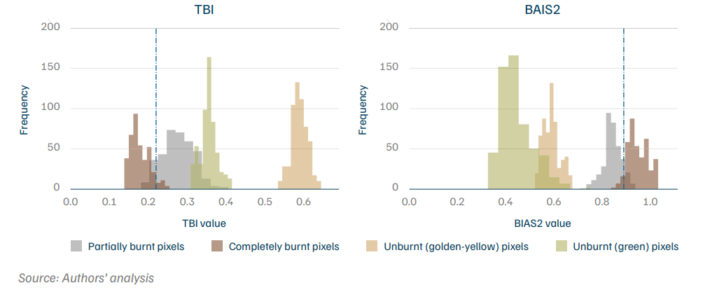
Figure 6. An overview of the data and methodology

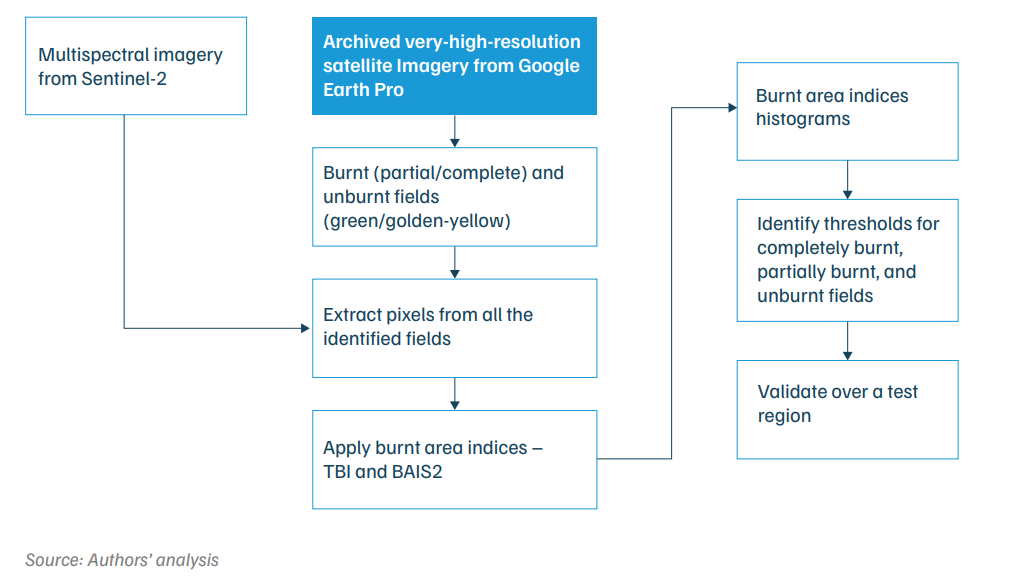
Figure 7. An overview of the methodology adopted for differentiating partially and completely burnt fields

FAQs

What are burnt area indices?

Burnt area indices are satellite data-based indicators that detect burnt fields by identifying changes in field characteristics before and after burning.
What are the limitations of remote sensing-based CRB monitoring?

Satellite-borne sensors can only detect active fires during the overpass. Coarse spatial and temporal resolution, obstruction due to clouds and smoke, are also challenges associated with remote sensing-based CRB monitoring.
What is the difference between partial and complete burning of fields?

In complete burning, the entire leftover straw after harvesting is set on fire, whereas in partial burning, only the loose straw left after running the harvester is burnt.
What are the implications of accurately monitoring CRB?

An accurate estimate of the extent of CRB helps assess the effectiveness of CRB mitigation policies. It will also help improve the emission estimates from CRB. In turn, this will lead to improvements in the performance of air quality models that run on these estimates.